This is a repost from my original reddit post. I’ve made a few changes to it to improve readability as well.
Introduction
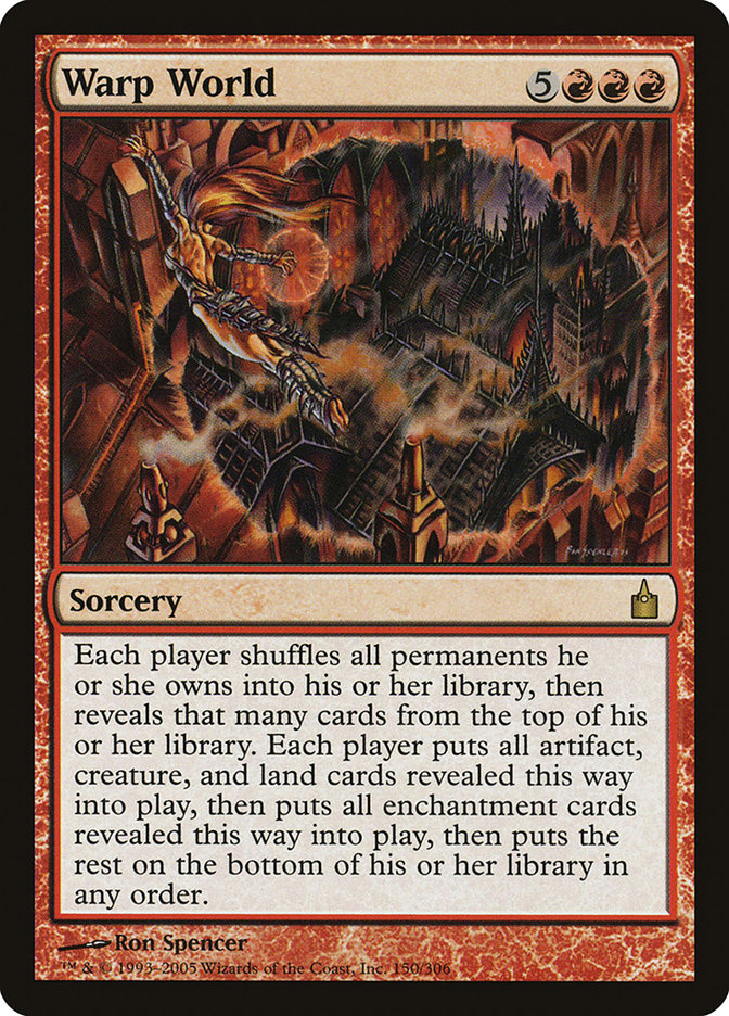
If you’re unfamiliar with Warp World, you are in for a treat. It’s a 5RRR sorcery from Ravnica that reads as follows:
Each player shuffles all permanents he or she owns into his or her library, then reveals that many cards from the top of his or her library. Each player puts all artifact, creature, and land cards revealed this way onto the battlefield, then does the same for enchantment cards, then puts all cards revealed this way that weren’t put onto the battlefield on the bottom of his or her library.
There are many different ways to build around such a card. For example, we can play mostly permanents in our deck (i.e., very few instants and sorceries), add creatures with enter the battlefield (ETB) ability (e.g., Eternal Witness), add creatures with landfall ability (Lotus Cobra), and so on. I’m not going to tell you how to play Warp World or advertise any particular deck that takes advantage of it. Instead, I’ll try to formalize what happens when we cast Warp World, and how the outcome of casting it changes as a function of the type of cards we choose to play and when we cast it.
This is not meant to be an exhaustive analysis of the card and all of its possible interactions. If you spot an error or thought about a much simpler way of analyzing Warp World, please feel free to share it. Above all, this is meant to be a mathematical and statistical exercise.
The Basics
In a game of magic, we play with a deck, Ω, composed of n cards, such that Ω = {ω1, …, ωn} is our deck. The current types of cards in MtG can be of two sorts, namely permanents (land, creature, artifact, enchantment, and planeswalker) and non-permanents (sorcery and instant). Let Λ be the set of all z permanents that we have in our deck (e.g., Elvish Mystic, forests, mountains, Primeval Titan), such that Λ = {λ1, …, λz} are all the permanents in our deck. Because there’re only permanents and non-permanents in our deck, the set of non-permanents can be defined as the negation of Λ, ¬Λ, such that ¬Λ ∪ Λ = Ω.
When a game of magic starts, our deck becomes our library. Let’s define our library by the set Θ of k cards, such that Θ = {θ1, …, θk} is our library, and the rules tell us that Θ ⊆ Ω, that is, all cards in our library are cards from our deck. In addition, when the game starts, it also creates other three zones that are of particular relevance to us, namely the battlefield, our hand, and the graveyard. Let’s define Ψ as the set of y permanents we have on the battlefield, such that Ψ = {ψ1, …, ψy} are the permanents we have on our side of the battlefield. To make matters as simple as possible for now, let’s also assume that Ψ ⊆ Λ, that is, all permanents we have on the battlefield are permanents from our deck, until otherwise specified, and permanents are all but planeswalkers. Then we define Α as the set of a permanents in our hand, such that Α = {α1, …, αa} are the permanents in our hand, and B is the set of b permanents in our graveyard, B = {β1, …, βb}. As before, let’s also assume that A ⊆ Λ and B ⊆ Λ.
Now we have a fairly good characterization of our deck and board state, so let’s see what Warp World does. First, it makes us:
- count all permanents we have on the battlefield;
- shuffle all of them into our library;
- then reveal as many cards from the top of our library as permanents we counted;
- and finally, put all revealed artifacts, creatures, lands, and (afterwards) enchantments onto the battlefield. Everything else that was not put onto the battlefield goes to the bottom of the library. (Our opponents do the same thing at the same time, and triggered abilities follow apnap order, as usual.)
Let’s relate what Warp World does to our previous definitions. During the first step, the number of permanents we have on the battlefield will be the cardinality of Ψ, that is, |Ψ| = y. During the second step, we put |Ψ ∩ Λ| cards back into our library, and because we’re assuming that Ψ ⊆ Λ, there are exactly y cards from Λ that will be put back into our library. So, by the end of the second step, our library will have exactly |Θ ∪ Ψ| = k + y cards, of which |Λ| - |Α ∪ B| = z - (a + b) are permanents. Regarding shuffling, we assume it’s not biased in any particular manner–that is, cards from our library are ordered at random every time it’s required to shuffle.
Here comes the interesting part, namely the third and fourth steps. During the third step, we’re instructed to reveal y cards from the top of our library and then, during the fourth step, we put all artifacts, creatures, lands, and enchantments revealed this way onto the battlefield. Let’s define Φ as the set of x revealed artifacts, creatures, lands, and enchantments, such that Φ = {φ1, …, φx} are all the revealed permanents that will be put onto the battlefield. Now, because we don’t know how all the cards in our library were ordered (unbiased shuffling), we can’t tell which cards will be revealed in a deterministic way (e.g., the first will be a land, the second will be a creature, etc.). Fortunately, we’re quite capable of telling which cards will be revealed in a stochastic way (probabilistically). For example, there’s a .90 chance to reveal a land, or there’s a .10 chance to reveal a creature.
The act of revealing cards from the top of our library is analogous to sampling objects from a finite population without replacing them, much like picking apples from an apple tree. Of note, we are usually revealing more than one card (y > 1), and for now, the outcomes of interest will fall into two main categories, namely it’s either a permanent that we will put onto the battlefield or not. If each sampling were independent of one another (e.g., after revealing a card, we reshuffle it back into our library before revealing another card), we could classify this action as a Bernoulli trial and compute the probability of revealing permanents according to the binomial distribution. However, in our case, each sampling is not independent of one another, as the probability of a success (to reveal a permanent) changes as the number of revealed cards also changes. Therefore, we should model such an action of revealing cards from the top of our library with a hypergeometric distribution, which some magic players should be already familiar with, as it is often used to compute the optimal number of lands in a deck, for example, or the chance of drawing a certain card by turn.
When there are two mutually exclusive outcomes (e.g., permanent and non-permanent card), the probability mass function (pmf) of the number of permanents that Warp World will reveal will take the form
in which (p ¦ q) is a binomial coefficient–that is, the number of ways q elements can be chosen from p elements, regardless of order, computed as p! / [q!(p - q)!]. Across four coin tosses (p = 4), for example, there are six different ways of arranging two Tails (q = 2)–namely, TTHH, THTH, THHT, HTTH, HTHT, and HHTT–which can be represented by the binomial coefficient (4 ¦ 2) = 6.
To make it easier for us, I wrote a table with definitions of the main parameters:
| parameter | definition |
|---|---|
| a | number of permanents in hand |
| b | number of permanents in the graveyard |
| k | number of cards in the library |
| x | number of permanents revealed with Warp World |
| y | number of cards revealed and number of permanents on the battlefield before resolving Warp World |
| z | number of permanents in the deck |
When we compute Eq.1 for all possible number of permanents revealed with Warp World, we get a probability distribution with mean
and variance
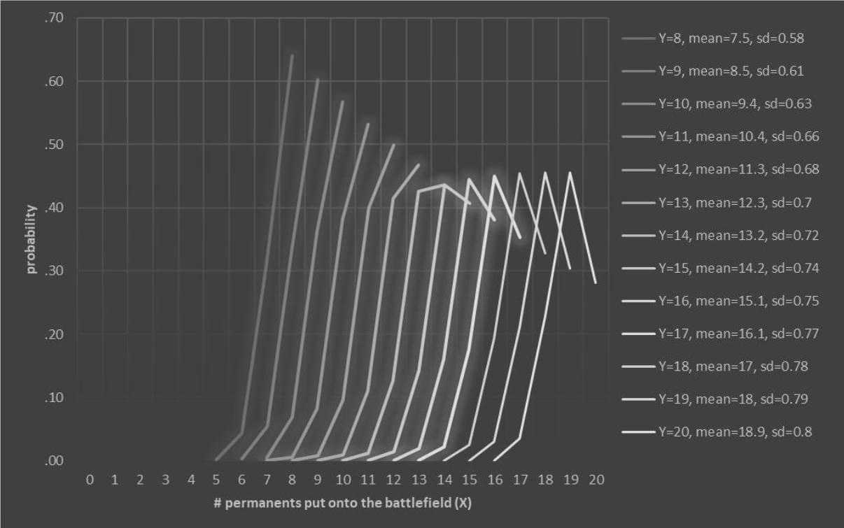
To illustrate its application, let’s imagine the following scenario. We’re playing with a 60-card deck that has 56 permanents (let’s think of them as all mountains; z = 56) and four copies of Warp World. The game starts. We’re on the play and we mull to two cards, a mountain and a copy of Warp World. During the next seven turns, we only draw mountains, so when we get to turn eight, we have eight mountains on the battlefield (y = 8), a single card in hand, which is Warp World, and 51 remaining cards in our library (k = 51). If we cast Warp World, what are our chances of putting, say, eight permanents back on the battlefield? What about seven, six, five, …? If we calculate such probabilities with Eq. 1 and plot the results for various numbers of permanents we had before casting Warp World (y), we get the following probability distributions:
In the horizontal axis, we have the number of permanents that we get after resolving Warp World (x), while in the vertical axis, we have the probability of each of them. In addition, the multiple distributions represent different numbers of permanents we had before casting Warp World (y). (Missing probabilities are all zero.) In our example, if we have 8 permanents on the battlefield when we cast Warp World, we will get a mean of 8 permanents after resolving Warp World—that is, we usually get our eight lands back—but if we have 20 permanents on the battlefield when we cast Warp World, on average, we get 19 permanents back. Notice that even though the variability (sd stands for standard deviation) is low in absolute terms (the value of x is likely equal or close to the mean), the higher is the value of y, the higher is the variance. For example, if we have 8 permanents on the battlefield, we will usually get 7 or 8 permanents after resolving Warp World, and rarely anything other than that. However, if we have 20 permanents on the battlefield, we will usually get something between 18 and 20 permanents after resolving Warp World, and rarely anything other than that.
Before we move on, I should point out that each probability in Figure 1 refers to the probability of getting exactly that number of permanents, as Eq. 1 is a pmf. However, if your interest is in answering questions about fewer-than/up-to/at-least a certain number of permanents, all you need to do is sum adjacent values of x in the appropriate direction to get the cumulative probability. For example, if we have 20 permanents on the board before casting Warp World, what would be the probability of getting at least, say, 18 permanents? According to the Y=20 distribution in Figure 1, that probability would be .96.
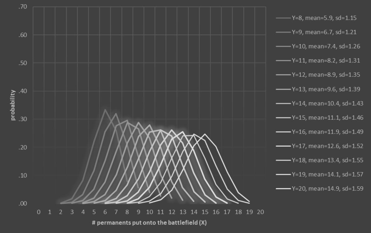
Despite being a somewhat unrealistic scenario, Figure 1 gives us something that we can use to compare against different situations. For instance, how adding more non-permanents to our deck would affect the previous distributions? Let’s set everything else equal to the previous example, except that now, our deck has 44 mountains (z = 44), four copies of Warp World, and 12 other non-permanents. The results are the following:
Inspection of Figure 2 indicates two main differences in comparison to Figure 1. First, adding more non-permanents to a Warp World deck decreases the mean of the probability distribution of the number of permanents you will get after resolving Warp World, regardless of how many permanents you had before casting Warp World. Second, variability increased all over the board, so the chance of getting screwed up by Warp World increased quite a lot. In other words, this is why it’s not a good idea to play non-permanents in a Warp World deck, as you decrease its expected value and increase its variability. You get double screwed.
The Multivariate Warp World Model
One limitation of the previous approach is that we can’t tell what sort of permanent Warp World puts onto the battlefield. In some cases, the binary distinction is just what we need. In others, however, a more detailed distinction is needed, as different types of permanent will have different effects on the board state after Warp World resolves. One distinction that would make sense is the one given by Warp World itself, namely that permanents can be artifacts, creatures, lands, and enchantments. We’ve already defined Λ as the set of all permanents in our deck, so it follows that artifacts, Λ1, creatures, Λ2, lands, Λ3, and enchantments, Λ4, ought to be subsets of Λ, such that
because for the sake of simplicity, we will continue to assume that we’re not playing planeswalkers. (Remember that Warp World does not put planeswalkers onto the battlefield, even though they are permanents that can be part of our deck.) Similarly, let’s say that mutually exclusive subsets of Φ, A, and B fall into the same categories as Λi, such that
Now we can extend Eq. 1 to accommodate the additional outcomes of Warp Wold as follows
which is the pmf of the multivariate Warp World model. Such a distribution has mean
and variance
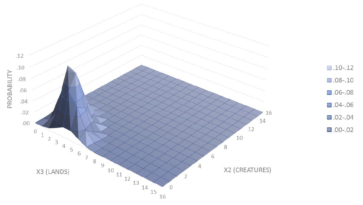
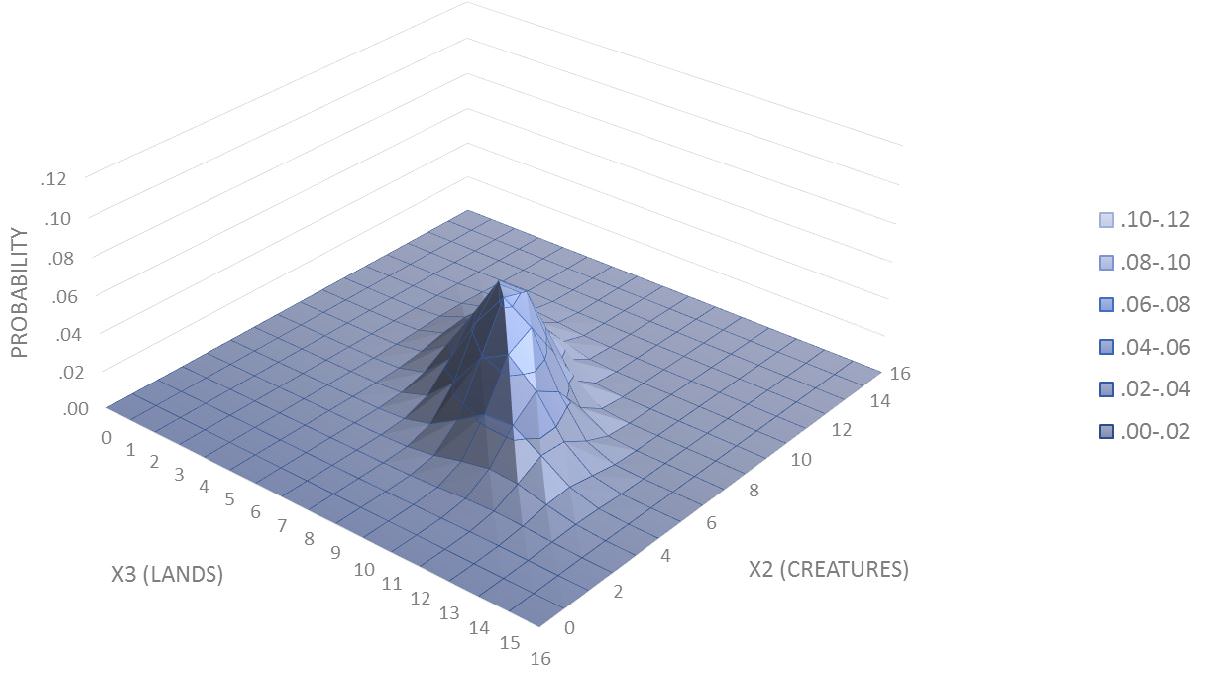
As before, let’s think about a scenario to illustrate how Eq. 4-6 informs us about the probability of Warp World revealing different sorts of permanents as a function of the properties of our deck. Similar to our previous example, imagine we we’re playing with a 60-card deck composed of 24 lands (z3 = 24), 16 creatures (z2 = 24), and 20 non-permanents. The game starts. We’re on the play and unfortunately, we have to mull to four cards, specifically two forests and two copies of Elvish Mystic. On turn 1, we play a forest and an elvish mystic. On turn 2, we draw a copy of Warp World, then play another forest and cast another elvish mystic. During the next four turns, we draw four mountains, so when we get to turn 6, we cast Warp World with two forests, four mountains, and two elvish mystics on the battlefield (y = 8), no cards in hand or graveyard, and 51 cards left in our library (k = 51). What’s the probability of revealing, say, two creatures and four lands with Warp World? On average, how many creatures and lands would Warp World put back on the battlefield after it resolves? We can answer such questions with Eq. 6-8. When we compute the probabilities in Eq. 6 for all possible values of x2 and x3 and plot such values, we generate the following three-dimensional representation of the probability distribution of x2 and x3
Figure 3 shows that when y = 8, the probability of revealing exactly two creatures and four lands from the top of our library is .10. In fact, this is one of the two most likely cases, the second one being two creatures and three lands, as both of them account for roughly 20% of the possible outcomes of a Warp World under this condition. In addition, Eq. 7 and 8 show that on average, Warp World will reveal 2 creatures (sd = 1 creature) and 3 lands (sd = 1 land) in this particular example.
We’ve seen before that playing non-permanents in a Warp World deck is a bad idea. So, let’s run the same simulation as before, except that instead of playing 16 creatures and 24 lands, our deck has 22 creatures and 26 lands. When that’s done, we find the following distribution
Inspection of Figure 4 indicates a shift of the mean of the probability distribution. Indeed, on average, Warp World would reveal 3 creatures (sd = 1 creatures) and 4 lands (sd = 1 lands) with the latter deck.
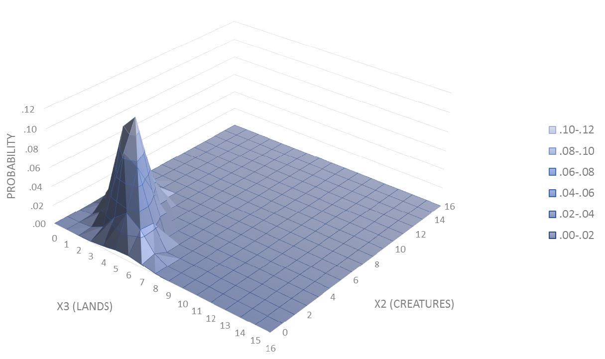
How would Figures 3 and 4 change if we increased the number of permanents on the battlefield before casting Warp World to, say, 20 permanents (y = 20)? The probability distribution of xi in Figure 3 would look like this
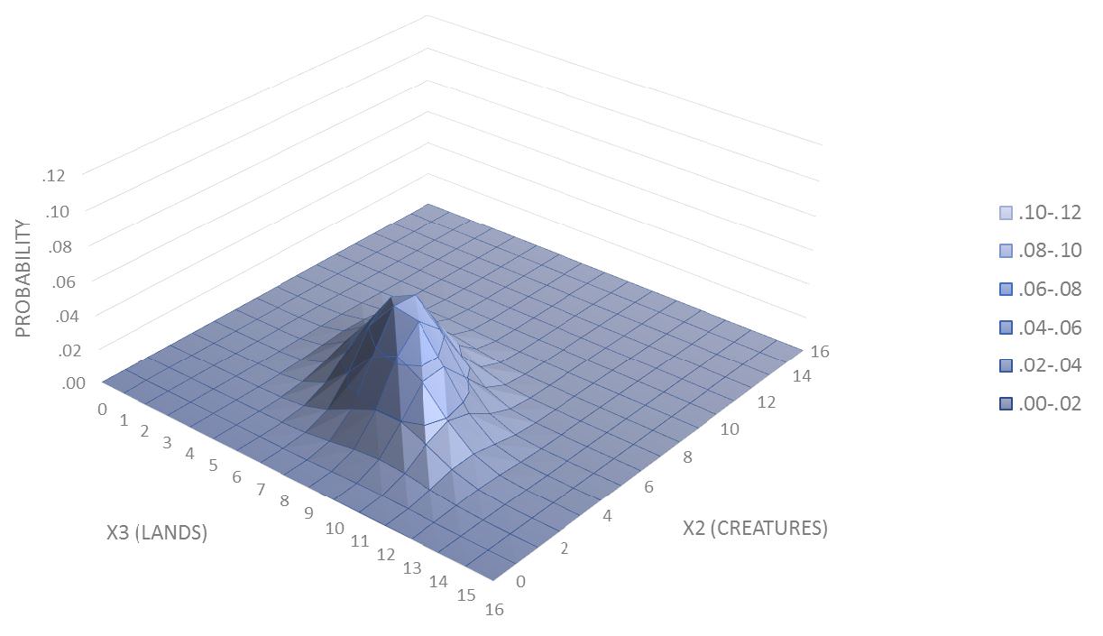
and would have mean 5 creatures (sd = 2) and 8 lands (sd = 2), while the distribution in Figure 4 would look like this
and have mean 8 creatures (sd = 2) and 9 lands (sd = 2).
Of course, we could calculate probability distributions for decks that have non-zero artifacts and enchantments as well but it would be difficult to visualize them, as we would be using higher dimensions than before. Similarly, the same approach could be used for different, mutually exclusive distinctions (e.g., green creatures vs. red creatures vs. other permanents; ramp permanents vs. graveyard recursion permanents).
There are many things that can be done moving forward. For instance, we could use Eq. 6-8 to investigate how cards that generate mana or produce more than one permanent can net mana or permanents, then describe the necessary and sufficient conditions to create loops with Warp World.
Tokens
So far, we’ve worked under the assumption that when we cast Warp World, the only sort of permanent we have on the battlefield (and thus the number of cards we will reveal with Warp World) are the ones contained in our deck—that is, Ψ ⊆ Λ. In some cases, this will be true; in others, however, it won’t, as we might have tokens on the battlefield, which will increase the number of cards revealed with Warp World but it doesn’t mean we’ll shuffle that many cards into our library. Fortunately, taking tokens into account does not require us to make huge changes to the previous equations. Specifically, if Ψ ⊆ Λ is not true, then by the end of the second step of Warp World, our new library will have size |Θ| + |Ψ ∩ Λ|, instead of |Θ ∪ Ψ|, in which Ψ ∩ Λ are all permanents on the battlefield that are permanents from our deck (i.e., all non-token permanents). Everything else remains the same.
Other Similar Spells
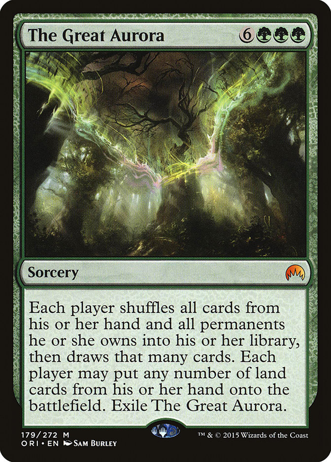
There are a few other spells that in one way or another, do something that is quite similar to what Warp World does. One example that comes to mind is The Great Aurora. I have no doubt we can use the Warp World model to compute probabilities for those spells as well. We just need to tweak the model a little bit to make it consistent with the wording used in similar spells (e.g., great aurora also makes we shuffle our hand).
Other Approaches
We could find probability distributions empirically. Goldfish a Warp World deck, say, a thousand times, take note of the relevant stats prior to and after casting Warp World, and estimate the distributions empirically.
Final Remarks
We end with a cautionary note. We know that adding more permanents to a Warp World deck usually yields a better outcome—that is, the more permanents we have in the deck, the more permanents we’ll likely reveal with Warp World. However, it would be inappropriate to simply compare mean differences to draw conclusions about different Warp World decks. That is because changing properties of Warp World decks will likely change the variance of their distributions. One possible solution is to use a standardized measure of the compound mean difference–that is, the standardized measure of distance between the means of two Pr(xi) distributions.

